• Step1:Loading the required packages and import the data
• Step2:Taking sample data from the whole data set
• Step3:Data Preparation : Scaling(Normalizing) the input data and filling the missing values.
• Step4:Finding the best Clustering Algorithm for our data set using two validation techniques internal and stability.
• Step6: Plotting the histogram of Flying Trans Miles using ggplot2
• Step7:Plotting FFP versus Enrollment duration and Flying Return Miles uisng ggplot2
• Step8:Computing Hierarchical Clustering and plotting dendrogram
• Step9:Compare the average values in each of the variables for the 2 clusters (the centroids of the clusters).

#Frequent Flyer program

#kmeans clustering

#Loading required pacakges

library(“xlsx”)
library(“openxlsx”) #Big excel file
library(“factoextra”) #Clustering Visualization
library(“dplyr”) # Data manipulation

#Input

input<-read.xlsx(“FlyerSample.xlsx”)
View(input)
str(input)
summary(input)

#Taking sample data

#set.seed(123)
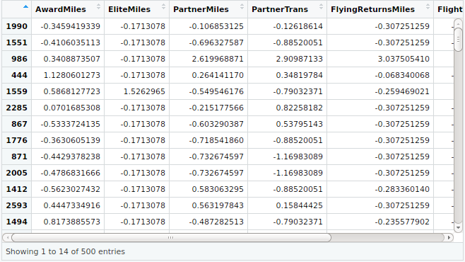
input1<-input[sample(nrow(input),500),]
View(input1)
str(input1)

#Data Preparation

#Checking Missing values

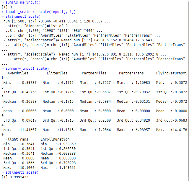
sum(is.na(input))

#Scaling the data

input1_scale<-scale(input1[,-1])
str(input1_scale)
summary(input1_scale)
sd(input1_scale)
View(input1_scale)

#Finding the best Clustering algorithm for our data

#install.packages(“clValid”)
library(clValid)

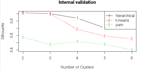
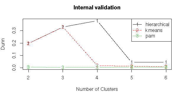
#Internal Validation Measures

#Compute clValid
clmethods<-c(“hierarchical”,”kmeans”,”pam”)
intern<-clValid(input1, nClust = 2:6,
clMethods = clmethods, validation = “internal”)
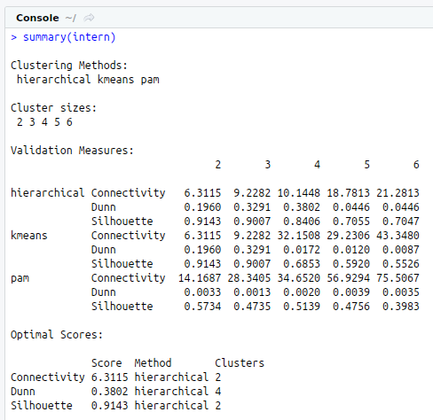
# Summary
summary(intern)

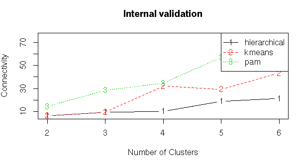
#Ploting the summary
plot(intern)

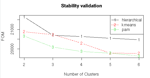
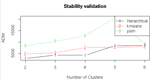
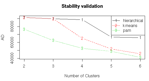
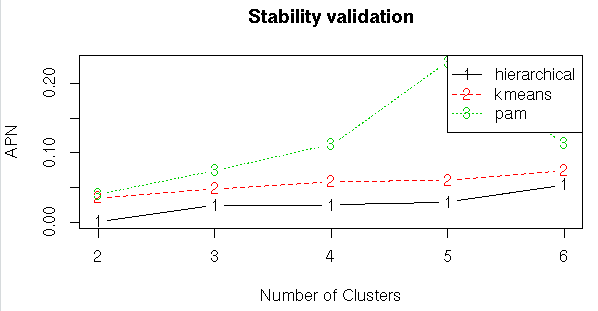
#Stability Validation Measures

stab<-clValid(input1,nClust=2:6,clMethods = clmethods,validation = “stability”)

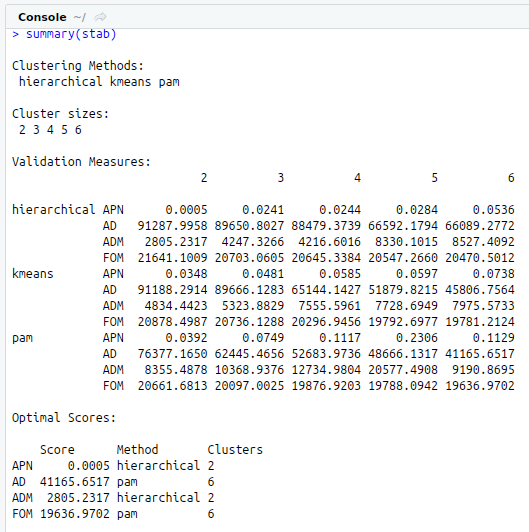
#Summary
summary(stab)

#Plotting the summary
plot(stab)

#Histogram of Flying Trans miles

library(“ggplot2”)
library(“ggpubr”)

ggplot(input1,aes(FlyingReturnsMiles),binwidth=50) + geom_histogram(fill= 678,boundary=150) + theme_pubclean() + ggtitle(“Number of flight miles in the past 12 months”)

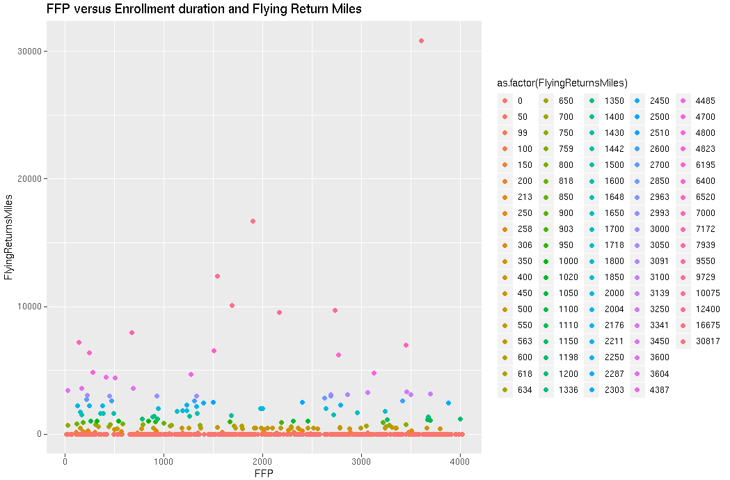
#FFP versus Enrollment duration and Flying Return Miles

ggplot(input1, aes(x=FFP,y=FlyingReturnsMiles,color=as.factor(FlyingReturnsMiles))) + geom_point() +
labs(title=”FFP versus Enrollment duration and Flying Return Miles”)

#Hierarchical Clustering

#Finding the more appropriate method for more strongest clustering structure

#install.packages(“purrr”)
library(“purrr”)

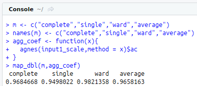
m<-c(“complete”,”single”,”ward”,”average”)
names(m)<-c(“complete”,”single”,”ward”,”average”)
agg_coef<-function(x){
agnes(input1_scale,method = x)$ac
}

map_dbl(m,agg_coef)

#Compute hclust
h_dist<-dist(input1_scale,method = “euclidean”)
h_data<-hclust(h_dist, method = “ward.D”)

#Plotting Dendrogram
#install.packages(“ggdendro”)
library(“ggdendro”)
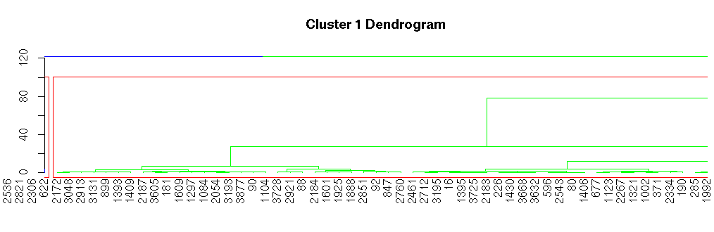
dend <-as.dendrogram(h_data) dend %>% set(“branches_k_color”,value=c(“blue”,”green”),k=2) %>% plot(main=”Cluster 1 Dendrogram”,xlim=c(90,140))
rect.hclust(h_data,k=2)
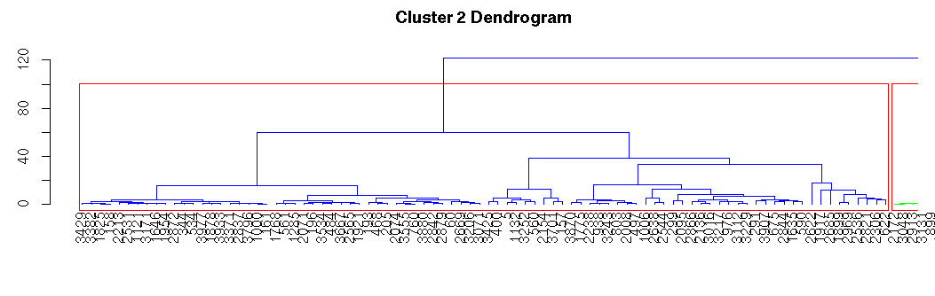
dend %>% set(“branches_k_color”,value=c(“blue”,”green”),k=2) %>% plot(main=”Cluster 2 Dendrogram”,xlim=c(1,88))
rect.hclust(h_data,k=2)

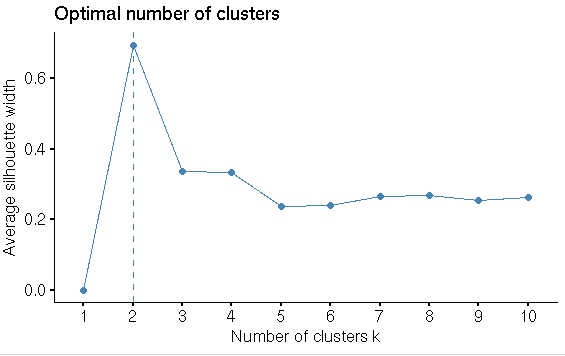
#Finding the optimal No of clusters
library(“factoextra”)

fviz_nbclust(input1_scale,hcut,method = “silhouette”)

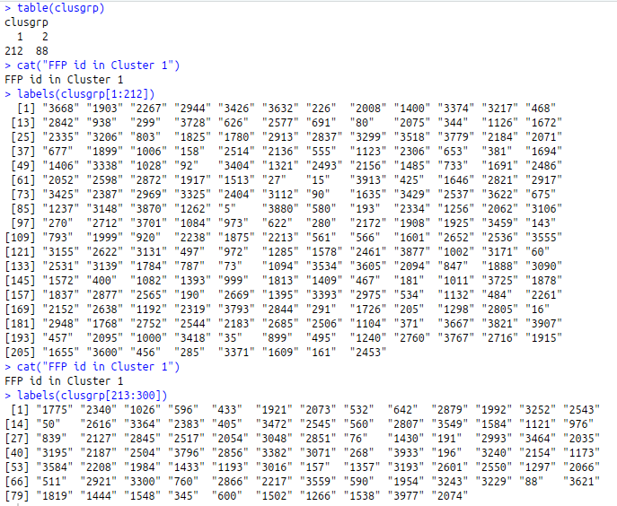
clusgrp<-cutree(h_data,k=2)
table(clusgrp)
cat(“FFP id in Cluster 1”)
labels(clusgrp[1:212])
cat(“FFP id in Cluster 1”)
labels(clusgrp[213:300])

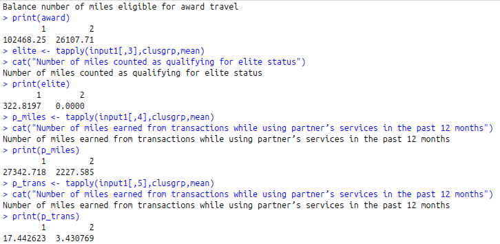
award<-tapply(input1[,2], clusgrp, mean)

cat(“Balance number of miles eligible for award travel\n”)
print(award)

elite<-tapply(input1[,3],clusgrp,mean)

cat(“Number of miles counted as qualifying for elite status”)
print(elite)

p_miles<-tapply(input1[,4],clusgrp,mean)

cat(“Number of miles earned from transactions while using partner’s services in the past 12 months”)
print(p_miles)

p_trans<-tapply(input1[,5],clusgrp,mean)

cat(“Number of miles earned from transactions while using partner’s services in the past 12 months”)
print(p_trans)

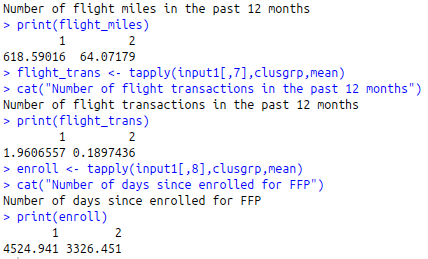
flight_miles<-tapply(input1[,6],clusgrp,mean)

cat(“Number of flight miles in the past 12 months”)
print(flight_miles)

flight_trans<-tapply(input1[,7],clusgrp,mean)

cat(“Number of flight transactions in the past 12 months”)
print(flight_trans)

enroll<-tapply(input1[,8],clusgrp,mean)

cat(“Number of days since enrolled for FFP”)
print(enroll)