Research Breakthrough Possible @S-Logix
Office Address
- 2nd Floor, #7a, High School Road, Secretariat Colony Ambattur, Chennai-600053 (Landmark: SRM School) Tamil Nadu, India
- pro@slogix.in
- +91-81240 01111
To implement the Logistic regression using R programming.
Step 1 : Import the data
Step 2 : Check Correlation
Step 3 : Splitting the data set into train and test
Step 4 : Create a relationship model for the train data using glm() function in R
Step 5 : Summary of the linear model using summary() function
Step 6 : Predicting the dependent variable for the test data using predict() function.
Step 7 : Plot the confusion matrix.
#Logistic Linear Regression Model
#Get and Set Working Directory
print(getwd())
setwd(“/home/soft13”)
getwd()
#Read file from Excel
#install.packages(“xlsx”)
library(“xlsx”)
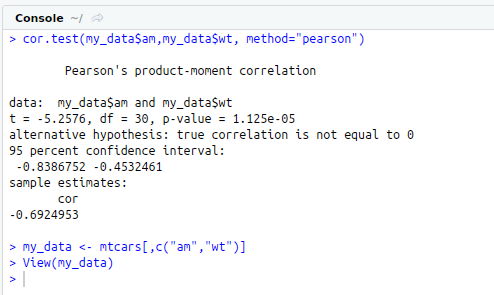
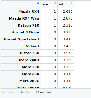
my_data<-mtcars[,c(“am”,”wt”)]
View(my_data)
#Correlation Test
cor.test(my_data$am,my_data$wt,method=”pearson”)
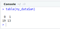
#Check class bias
table(my_data$am)
#Splitting into train and test data manually
#Train data
train_one<-my_data[which(my_data$am==1),]
train_zero<-my_data[which(my_data$am==0),]
train_1<-sample(1:nrow(train_one), 0.7*nrow(train_one))
train_0<-sample(1:nrow(train_zero), 0.7*nrow(train_zero))
training_1<-train_one[train_1,]
training_0<-train_zero[train_0,]
train<-rbind(training_1,training_0)
#Test data
testing_1<-train_one[-train_1,]
testing_0<-train_zero[-train_0,]
test<-rbind(testing_1,testing_0)
#Logistic Regression
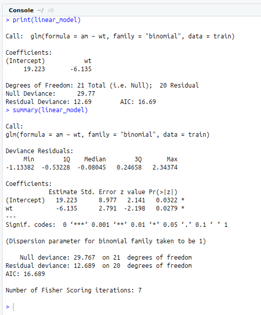
linear_model<-glm(am ~ wt,data = train,family=”binomial”)
print(linear_model)
summary(linear_model)
#Prediction
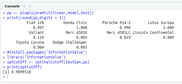
pp<-plogis(predict(linear_model,test))
print(round(pp,digits = 3))
#Optimal Cut-off
#install.packages(“InformationValue”)
library(“InformationValue”)
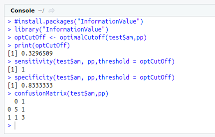
optCutOff<-optimalCutoff(test$am,pp)
print(optCutOff)
#Sensitivity
sensitivity(test$am, pp)
#Specificity
specificity(test$am, pp,threshold = optCutOff)
#ConfusionMatrix
confusionMatrix(test$am,pp)