What is Time Series Analysis?

• Time series analysis comprises methods for analyzing time series data in order to extract meaningful statistics and other characteristics of the data.
• Time series forecasting is the use of a model to predict future values based on previously observed value.

Data set :

• AirPassengers – R inbuilt dataset

R Packages :

• ggfortify — Fior Visualization
• tseries – To implement Time Series
• forecast – To implement Forecasting

R Function:

• autoplot(data) – It is a generic function to visualize various data object,
• decompose(data,type= ) – To Decompose a time series into seasonal, trend and irregular components

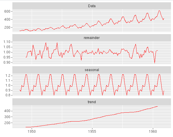
type – Addictive, Multiplicative which is the seasonal component

• adf.test(data) – Function for Augmented Dickey Fuller test

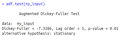
H0: Time Series object is not stationary

H1 : Time Series object is stationary

• auto.arima(ts_object) – To implement time series model
• forecast(fitted model,h=) – To implement forecasting

#Import Data

my_input<-AirPassengers
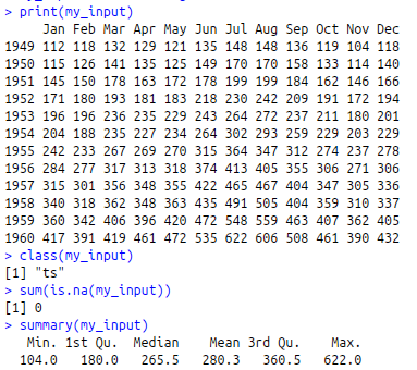
print(my_input)
class(my_input)

#Check for Missing Values

sum(is.na(my_input))

#Summary

summary(my_input)

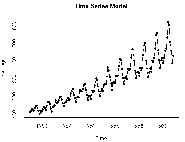
#Plot Time Series

plot(my_input,ylab=”Passengers”,main=”Time Series Model”,type=”o”,pch=19,cex=0.8)

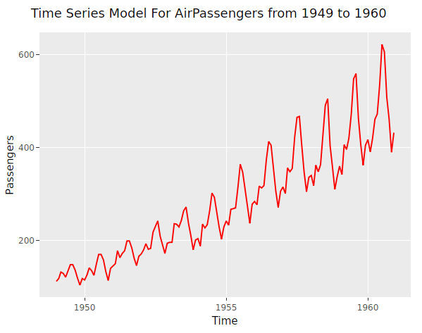
#Plotting using ggplot2 to see the trend

#install.packages(“ggfortify”)
library(“ggfortify”)

gb<-autoplot(my_input,fill=”red”) + labs(title=”Time Series Model For AirPassengers from 1949 to 1960″,x=”Time”,y=”Passengers”)

#install.packages(“plotly”)
library(“plotly”)
ggplotly(gb)

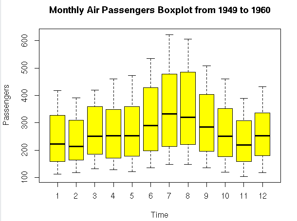
#Box Plot to see Seasonal Effects

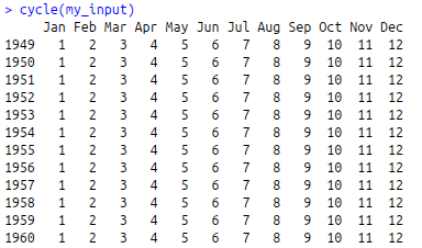
cycle(my_input)
boxplot(my_input~cycle(my_input),xlab=”Time”,ylab=”Passengers”,main=”Monthly Air Passengers Boxplot from 1949 to 1960″,col=”yellow”)

#Decompose the Time Series

decom_time<-decompose(my_input,type=”multiplicative”)
autoplot(decom_time,fill=”red”)

#Test Stationarity of the Time Series

#Using Augmented Dickey- Fuller test

#install.packages(“tseries”)
library(“tseries”)
adf.test(my_input)

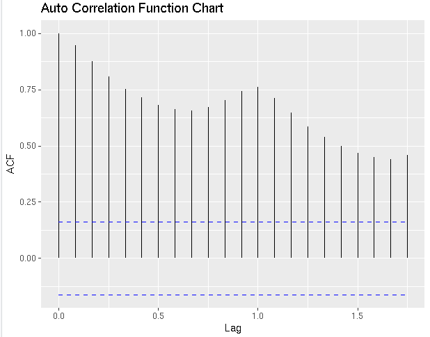
#Using ACF chart

autoplot(acf(my_input)) + labs(title=”Auto Correlation Function Chart”)

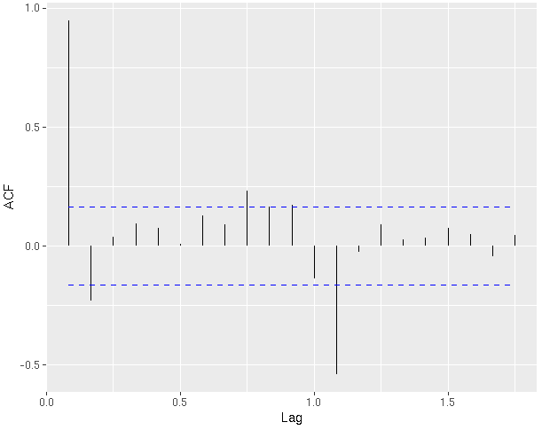
autoplot(pacf(my_input))

#Fit a time Series model

#ARIMA model

#install.packages(“forecast”)
library(“forecast”)
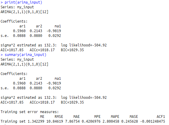
arima_input<-auto.arima(my_input)
print(arima_input)
summary(arima_input)

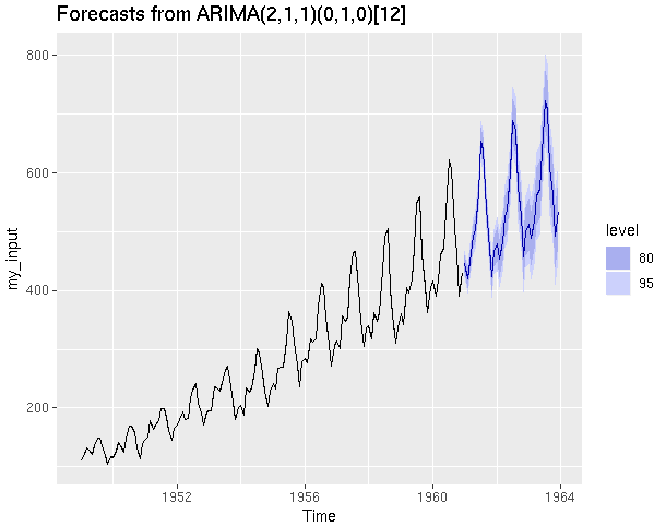
#Calculate Forecasts

fore_input<-forecast(arima_input,h=36,level = c(80,95))
autoplot(fore_input)