Research Breakthrough Possible @S-Logix
Office Address
- 2nd Floor, #7a, High School Road, Secretariat Colony Ambattur, Chennai-600053 (Landmark: SRM School) Tamil Nadu, India
- pro@slogix.in
- +91-81240 01111
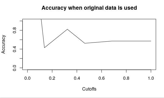
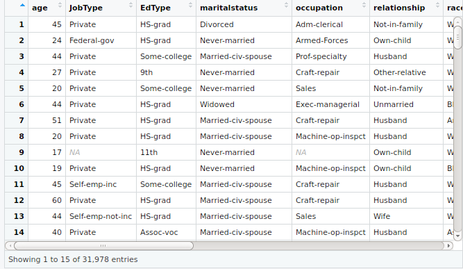
To predict the income for the given data set using logistic regression in R.
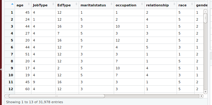
Step 1: Load the data
Step 2: Data Preparation : Filling Missing values and Outliers
Step 3: Replacing factor with a numeric value using plyr package
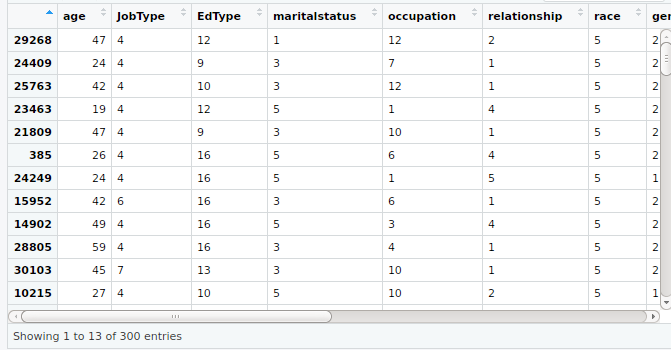
Step 4: Taking sample data from the whole data set
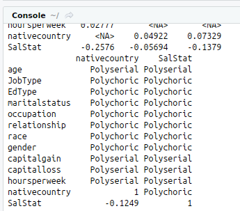
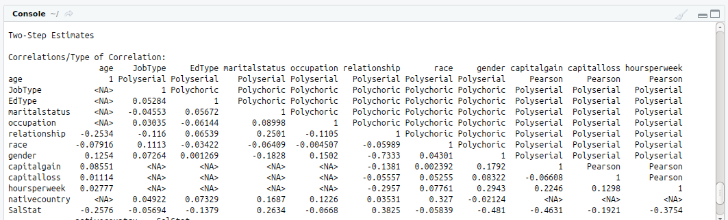
Step 5: Finding Correlation between variables
Step 6: Splitting the data into train and test data set
Step 7: Building the Regression Model
Step 8: Prediction
Step9: Confusion Matrix
#Loading input from an excel file
#install.packages(“xlsx”)
library(“xlsx”)
library(“openxlsx”) #For big Excel File
data.frame<-read.xlsx(“IncomePrediction.xlsx”,sheet = 1)
input<-data.frame
View(input)
#Data Preparation
#Filling Missing Value with Mode
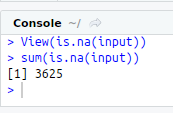
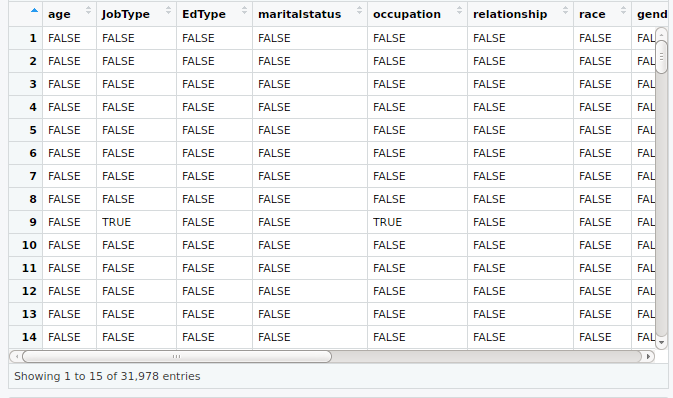
View(is.na(input))
sum(is.na(input))
mode<-function(f){
uniq<-unique(f)
uniq[which.max(tabulate(match(f,uniq)))]
}
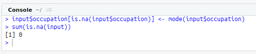
input$JobType[is.na(input$JobType)]<-mode(input$JobType)
input$occupation[is.na(input$occupation)]<-mode(input$occupation)
sum(is.na(input))
#Resolving Outlier
#Box Polot with Outliers
#install.packages(“plotly”)
library(“plotly”)
g<-ggplot(input,aes(x=input$SalStat,y=input$age,fill=input$SalStat)) + geom_boxplot() + ggtitle(“Box Plot Of Salary Status versus Age”) + xlab(“Salary Status”) + ylab(“Age”)
ggplotly(g)
boxplot(input$age,col = “red”,main=”Box Plot with outliers”)
#Replacing outlier with values
remove_outliers<-function(x,na.rm=TRUE) {
qnt<-quantile(x, probs=c(.25, .75))
caps<-quantile(x,probs = c(0.05,0.95),na.rm = na.rm)
H x[x < (qnt[1] – H)]<-caps[1] x[x > (qnt[2] + H)]<-caps[2]
x
}
input$age<-remove_outliers(input$age)
boxplot(input$age,col = “red”,main=”Box Plot without outliers”)
#Replacing Factor with a numeric value
#install.packages(“plyr”)
library(“plyr”)
job_fact<-factor(input$JobType)
ed_fact<-factor(input$EdType)
mar_fact<-factor(input$maritalstatus)
occ_fact<-factor(input$occupation)
rel_fact<-factor(input$relationship)
race_fact<-factor(input$race)
gen_fact<-factor(input$gender)
native_fact<-factor(input$nativecountry)
sal_fact<-factor(input$SalStat)
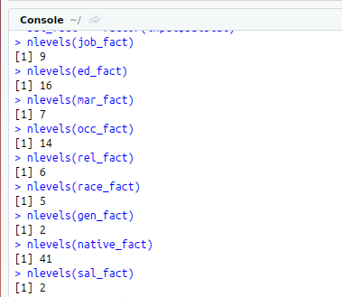
nlevels(job_fact)
nlevels(ed_fact)
nlevels(mar_fact)
nlevels(occ_fact)
nlevels(rel_fact)
nlevels(race_fact)
nlevels(gen_fact)
nlevels(native_fact)
nlevels(sal_fact)
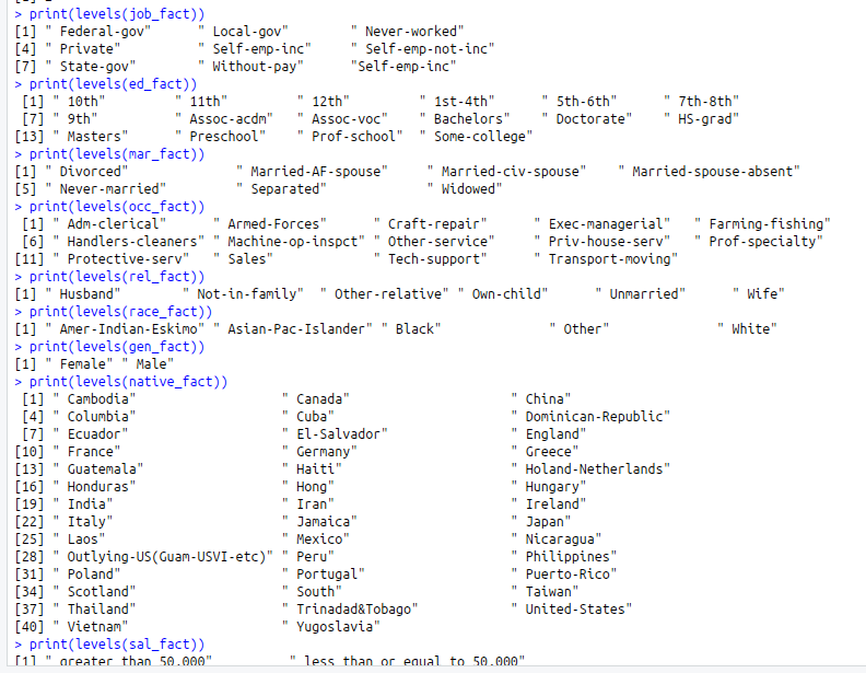
print(levels(job_fact))
print(levels(ed_fact))
print(levels(mar_fact))
print(levels(occ_fact))
print(levels(rel_fact))
print(levels(race_fact))
print(levels(gen_fact))
print(levels(native_fact))
print(levels(sal_fact))
input$JobType input$EdType<-mapvalues(ed_fact,from = c(” 10th”,” 11th”, ” 12th”, ” 1st-4th” , ” 5th-6th”, ” 7th-8th”,” 9th” ,” Assoc-acdm”,” Assoc-voc”,” Bachelors”, ” Doctorate”,” HS-grad”,” Masters”,” Preschool”, ” Prof-school”, ” Some-college”),to=c(1:16))
input$maritalstatus input$occupation input$relationship input$race input$gender input$nativecountry input$SalStat View(input)
#Taking sample data from whole dataset
set.seed(300)
input1<-input[sample(nrow(input),300),]
View(input1)
write.xlsx(input1, “IncomeSampleData.xlsx”)
View(input1)
#Correlation
#install.packages(“polycor”)
library(“polycor”)
hetcor(input1)
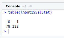
#Check class bias
table(input1$SalStat)
#Splitting into Train and test data
set.seed(301)
training_1<-input1[which(input1$SalStat==0),]
training_2<-input1[which(input1$SalStat==1),]
train_1<-sample(1:nrow(training_1),0.8*nrow(training_1))
train_2<-sample(1:nrow(training_2),0.8*nrow(training_2))
train_one<-training_1[train_1,]
train_two<-training_2[train_2,]
#Train data
train<-rbind(train_one,train_two)
#Test Data
test_one<-training_1[-train_1,]
test_two<-training_2[-train_2,]
test<-rbind(test_one,test_two)
#Logit model
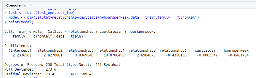
model<-glm(SalStat~relationship+capitalgain+hoursperweek,data = train,family = “binomial”)
print(model)
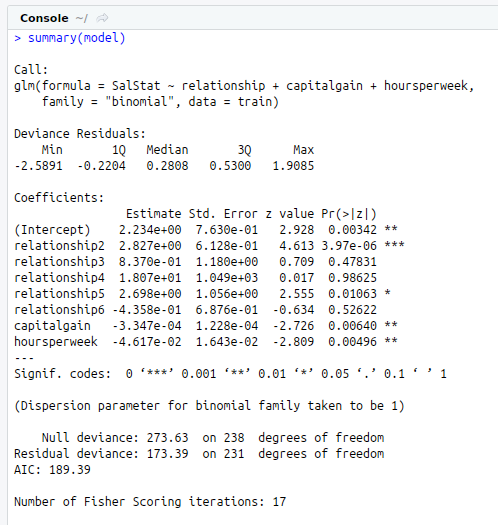
summary(model)
#Prediction
pp<-round(predict(model,test,type=’response’),digits = 0)
#Confusion Matrix
#install.packages(“caret”)
library(“caret”)
#install.packages(“e1071”)
library(“e1071”)
levels(as.factor(pp))
confusionMatrix(test$SalStat,as.factor(pp))