Load the required libraries

  Load the data set

  Compute the Principal Component Analysis

  Create a data frame with desired number of principal component(This can be done by Analyzing the summary of the PCA(Proportion of variance or Cumulative proportion))

  Split this data frame for train and test

  Build the model using train and predict using the test data

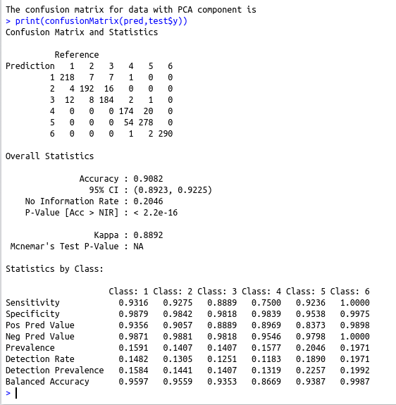
  Compute the confusion Matrix

  Create another data frame for the original data

  Split this data frame for train and test

  Build the model using train and predict using the test data

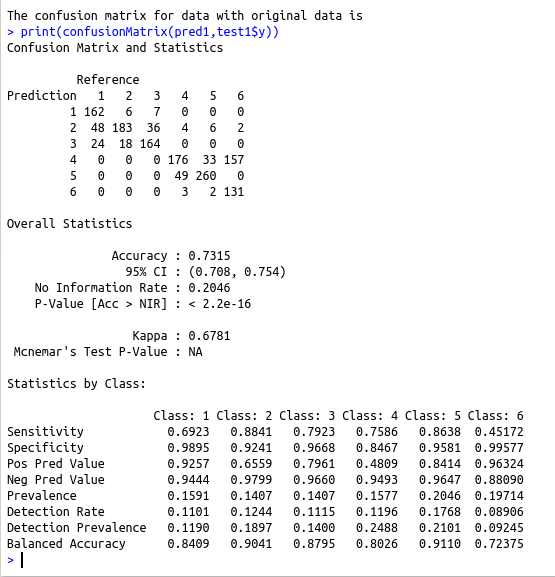
  Compute the confusion matrix

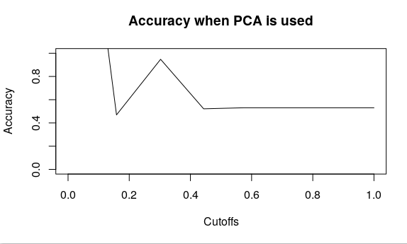
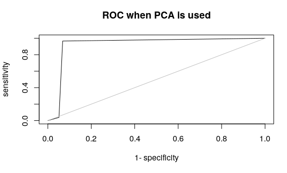
  Compare the confusion matrix obtained from the two model and interpret the result

#load the required libraries
require(MASS)
library(caret)
library(naivebayes)
library(AUC)
#Load the data set
data=read.csv(‘/…../X_train.txt’,header=FALSE,sep=””)
y=read.csv(‘/home/soft23/Downloads/UCI HAR Dataset/train/y_train.txt’,header=FALSE)
#To Split 80% of data as training data
smp_size train_ind #Compute the Principal component Analysis
pca_HAR summary(pca_HAR)
##Create the dataframe with PCA component and y
final_data=data.frame(x=pca_HAR$x[,1:70],y=as.factor(y$V1))
##Split the PCA dataframe for train and test
train test #Build the naive bayes model using the PCA component
nb #Predict using the test data of PCA component
pred=predict(nb,test)
#Compute the confusion matrix
cat(“The confusion matrix for data with PCA component is \n”)
print(confusionMatrix(pred,test$y))
#Create data frame with x and y original data
##Here X and y are in different file so we are creating a data frame to combine them
##In case if the x and y are in single file this step can be skipped
final_data1=data.frame(x=data,y=as.factor(y$V1))
#Split the data for train and test
train1 test1 #Build the naive bayes model using the original train data
nb1 #Predict using the original test data
pred1=predict(nb1,test1)
#Compute the confusion matrix
cat(“The confusion matrix for data with original data is \n”)
print(confusionMatrix(pred1,test1$y))
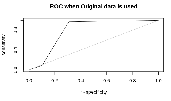
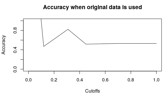
#To interpret the result
plot(accuracy(pred,test$y), type = “l”,main=”Accuracy when PCA is used”)
plot(accuracy(pred1,test1$y), type = “l”,main=”Accuracy when original data is used”)
plot(roc(pred,test$y), type = “l”,main=”ROC when PCA is used”)
plot(roc(pred1,test1$y), type = “l”,main=”ROC when Original data is used”)