How to Classify Weather Types Using a GRU Neural Network Model
Share
Condition for Classifying Weather Types Using a GRU Neural Network
Description: A GRU-based neural network to classify weather types using a weather dataset. It preprocesses the data by encoding categorical variables, scaling features, and reshaping the input for the GRU model. The model is trained, evaluated, and visualized using metrics such as accuracy, F1 score, and a confusion matrix heatmap.
Step-by-Step Process
Import Libraries: Essential libraries such as Pandas, Numpy, TensorFlow, and Scikit-Learn are imported for data preprocessing, model building, and evaluation. Visualization libraries like Matplotlib and Seaborn are included for plotting.
Load and Inspect Dataset: The weather classification dataset is loaded using Pandas' read_csv() function. It contains various features related to weather and the target variable 'Weather Type.'
Check for Missing Data: The dataset is checked for null and NaN values using isnull().sum() to ensure data completeness before proceeding with further steps.
Visualize Correlations: The correlation matrix is computed and visualized using Seaborn's heatmap. This helps identify relationships between features and detect possible redundancies.
Prepare Data: The feature set (x) is prepared by dropping the target column, and the target variable (y) is set to 'Weather Type.' Categorical variables in x are label-encoded to convert them into numerical form.
Encode Target Variable: The target variable 'Weather Type' is encoded into numeric labels using LabelEncoder(). A list of unique weather types is stored for future reference.
Scale Features: The features are scaled using StandardScaler() to standardize data, improving model performance. The input is reshaped to a 3D array suitable for the GRU model.
Train-Test Split: The dataset is split into training and testing sets using an 80:20 ratio with train_test_split(). This ensures a separate set of data for model evaluation.
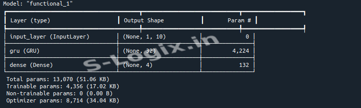
Build and Train GRU Model: A GRU-based neural network is defined with an input layer, a GRU layer, and a dense output layer. It is trained for 10 epochs with a batch size of 2.
Evaluate and Visualize: Predictions are made on the test set, and evaluation metrics such as accuracy, F1 score, recall, and precision are computed. A confusion matrix is plotted to visualize classification results.
Sample Source Code
# Import Necessary Libraries
import pandas as pd
import numpy as np
import matplotlib.pyplot as plt
import seaborn as sns
from sklearn.preprocessing import LabelEncoder, StandardScaler
from sklearn.model_selection import train_test_split
from tensorflow.keras.layers import Dense, Input, GRU
from tensorflow.keras.models import Model
from sklearn.metrics import (classification_report, confusion_matrix, accuracy_score, f1_score, recall_score, precision_score)
 Research Breakthrough Possible @S-Logix