List of Topics:
Location Research Breakthrough Possible @S-Logix pro@slogix.in

Office Address

Social List

How to Build and Evaluate a Deep Neural Network for Binary Classification Based on Customer Response Prediction

Building and Evaluating a Deep Neural Network for Binary Classification in Customer Response Prediction

Condition for Building and Evaluating a Deep Neural Network for Binary Classification in Customer Response Prediction

  • Description:
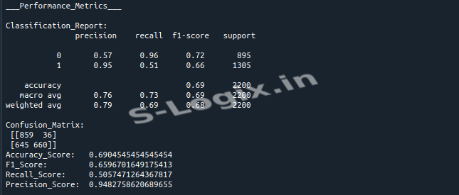
    The code preprocesses a dataset for binary classification by handling missing values and scaling features. It then builds a deep neural network (DNN) with dropout layers for regularization, trains it on the processed data, and evaluates the model using various performance metrics. The results include a confusion matrix and detailed classification metrics such as accuracy, F1 score, and precision.
Step-by-Step Process
  • Import the dataset:
    Import the dataset and display the first few rows to understand its structure. Check for missing and null values in the dataset.
  • Convert categorical columns:
    Convert categorical columns with object data type into numeric values using LabelEncoder for model processing.
  • Visualize class distribution:
    Use a count plot to visualize the distribution of the target variable (binary class) and check for class imbalance.
  • Compute and visualize correlation:
    Compute and visualize the correlation matrix of features using a heatmap.
  • Feature scaling:
    Standardize the features using StandardScaler to improve model performance.
  • Split the data:
    Split the data into training and testing sets using train_test_split to evaluate the model’s performance on unseen data.
  • Define DNN model:
    Define the DNN architecture with two hidden layers, each followed by a dropout layer for regularization.
  • Train and evaluate the model:
    Train the DNN model using the Adam optimizer and binary cross-entropy loss function. Evaluate using validation data.
  • Evaluate on test set:
    After training, evaluate the model on the test set using classification metrics (accuracy, F1 score, recall, precision) and display a confusion matrix.
Sample Source Code
  • # Import Necessary Libraries
    import pandas as pd
    from sklearn.preprocessing import LabelEncoder, StandardScaler
    import seaborn as sns
    import matplotlib.pyplot as plt
    from sklearn.model_selection import train_test_split
    from tensorflow.keras.layers import Dense, Input, Dropout
    from tensorflow.keras.models import Model
    from sklearn.metrics import (classification_report, confusion_matrix, accuracy_score, f1_score, recall_score, precision_score)

    df = pd.read_csv("/home/soft12/Downloads/sample_dataset/Website/Dataset/Train.csv")

    # Check Nan values
    print("Check Nan values")
    print(df.isna().sum())

    # Check Null values
    print("Check Null values\n")
    print(df.isnull().sum())

    label = LabelEncoder()

    # Convert object dtype into numeric
    for i in df.columns:
    if df[i].dtypes == 'object':
    df[i] = label.fit_transform(df[i])

    # Check class imbalance
    plt.figure(figsize=(6, 4))
    sns.countplot(x='Reached.on.Time_Y.N', data=df, palette='viridis')
    plt.title('Class Distribution')
    plt.xlabel('Class')
    plt.ylabel('Count')
    plt.show()

    # Compute the correlation matrix
    correlation_matrix = df.corr()
    # Display the correlation matrix
    print(correlation_matrix)

    # Plot the heatmap
    plt.figure(figsize=(10, 8))
    sns.heatmap(correlation_matrix, annot=True, cmap='coolwarm', fmt='.2f', linewidths=0.5)
    plt.title('Correlation Heatmap')
    plt.show()

    x = df.drop('Reached.on.Time_Y.N', axis=1)
    y = df['Reached.on.Time_Y.N']

    # Scaling the input data
    scaler = StandardScaler()
    x = scaler.fit_transform(x)

    # Split the train_test_data
    X_train, X_test, y_train, y_test = train_test_split(x, y, test_size=.2, random_state=42)

    def DNN_model(input_shape):
    # Input layer
    inputs = Input(shape=(input_shape,))
    # Hidden layers
    layer1 = Dense(64, activation='relu')(inputs)
    drop1 = Dropout(0.2)(layer1)
    layer2 = Dense(32, activation='relu')(drop1)
    drop2 = Dropout(0.2)(layer2)
    # Output layer
    output_layer = Dense(1, activation='sigmoid')(drop2)

    # Build the model
    ann_model = Model(inputs=inputs, outputs=output_layer)

    # Compile the model with Adam optimizer and binary crossentropy loss function
    ann_model.compile(optimizer='adam', loss='binary_crossentropy', metrics=['accuracy'])

    return ann_model

    model = DNN_model(X_train.shape[1])

    # Summary of Model
    model.summary()

    model.fit(X_train, y_train, batch_size=2, epochs=10, validation_data=(X_test, y_test))

    y_pred = model.predict(X_test)
    y_pred = [1 if i > 0.5 else 0 for i in y_pred]

    # Calculate confusion matrix
    cm = confusion_matrix(y_test, y_pred)

    class_labels = ['0', '1']

    # Plot the heatmap with correct labels
    plt.figure(figsize=(6, 5))
    sns.heatmap(cm, annot=True, fmt='d', cmap='Blues', xticklabels=class_labels, yticklabels=class_labels)
    plt.title('Confusion Matrix Heatmap')
    plt.xlabel('Predicted Label')
    plt.ylabel('True Label')
    plt.show()

    print("___Performance_Metrics___\n")
    print('Classification_Report:\n', classification_report(y_test, y_pred))
    print('Confusion_Matrix:\n', confusion_matrix(y_test, y_pred))
    print('Accuracy_Score: ', accuracy_score(y_test, y_pred))
    print('F1_Score: ', f1_score(y_test, y_pred))
    print('Recall_Score: ', recall_score(y_test, y_pred))
    print('Precision_Score: ', precision_score(y_test, y_pred))
Screenshots
  • DNN Output Screenshot